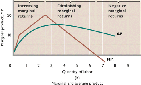
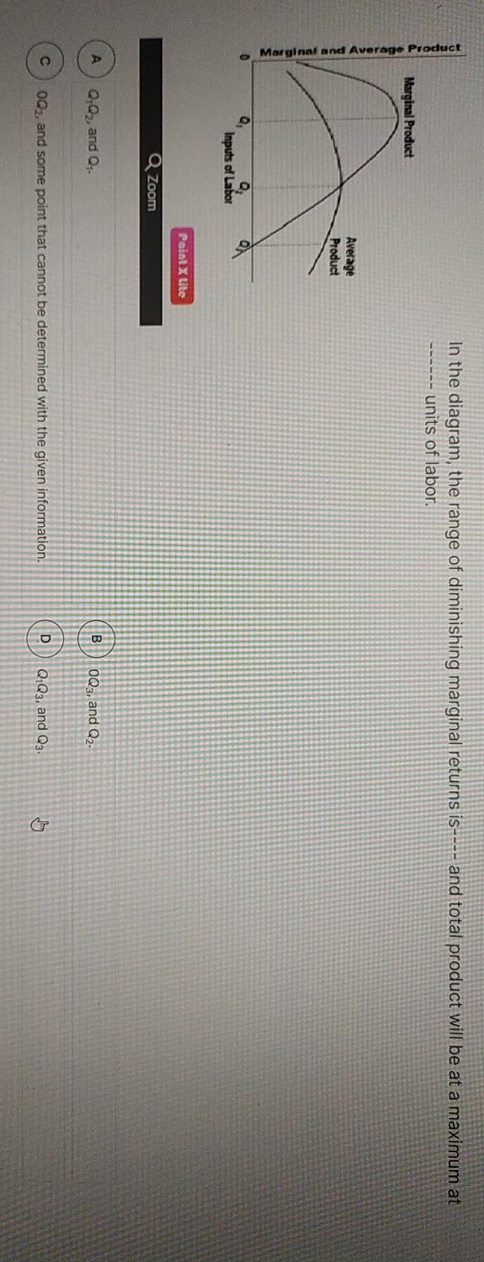
39 in the diagram, the range of diminishing marginal returns is
Solved > 41.The short run is characterized by: A. plenty ... In the above diagram the range of diminishing marginal returns is: A. 0Q3. B. 0Q2. ... 71.Marginal cost is the: A. rate of change in total fixed cost that results from producing one more unit of output. The Law of Diminishing Marginal Returns - Economics Help As extra workers produce less, the MC increases. Diagram of diminishing returns In this example, after three workers, diminishing returns sets in. After employing 4 workers or more - the marginal product (MP) of the worker declines and the marginal cost (MC) starts to rise. Difference between diminishing returns and dis-economies of scale
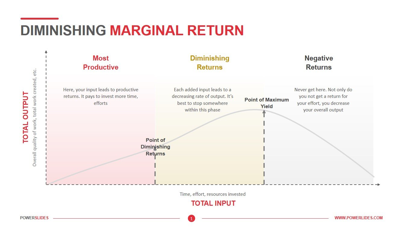
Law of Diminishing Marginal Returns (Definition and 3 ... Diminishing Marginal Returns Diagram As we can see from the diagram, at 3 workers, the gap between marginal profit and marginal cost is at its maximum. However, at 4 workers, the marginal cost of producing an additional unit starts to become more expensive. At this point, we start to see diminishing marginal returns.

In the diagram, the range of diminishing marginal returns is
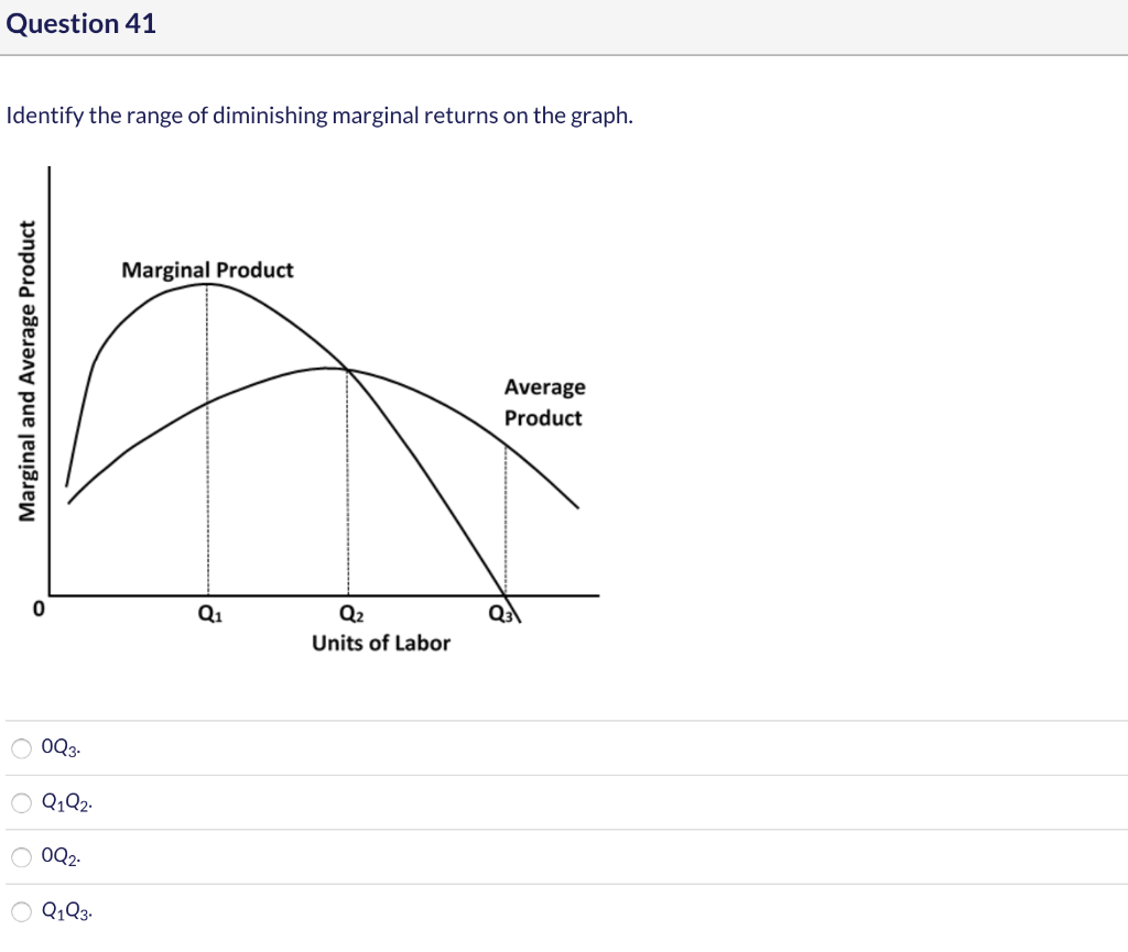
econ exam #2 Flashcards - Quizlet In the above diagram the range of diminishing marginal returns is: Q1Q3. In the above diagram, total product will be at a maximum at: Q3 units of labor. Refer to the above diagram. At output level Q total variable cost is: ... The above diagram indicates that the marginal revenue of the sixth unit of output is. not 4. tutor2u | Law of Diminishing Returns, Marginal Cost and ... Diminishing returns to labour in the short run. As more of a variable factor (e.g. labour) is added to a fixed factor (e.g. capital), a firm will reach a point where it has a disproportionate quantity of labour to capital and so the marginal product of labour will fall, thus raising marginal cost and average variable cost. The Production Process (With Diagram) - Economics Discussion Over this range marginal product is diminishing. 4. Finally, a point will be reached beyond which total output itself will actually fall, indicating a negative marginal product. In Fig. 13.4, this occurs for employment levels greater than 5.6. iii. The Average-Marginal Relationship: There is also a very close relation between MP L and AP L.
In the diagram, the range of diminishing marginal returns is. Assignment Topic: DIMINISHING MARGINAL RETURNS - My ... The diagram above shows the diminishing marginal returns as the number of workers are increased but the land and other factors are kept constant (Gillespie, 2011). As shown after a certain number of workers is increased the output first increases at a lower rate and after some time it starts declining. The Law of Diminishing Return Definition, Graph | Study ... The law of diminishing return indicates that if the number of variable inputs is increased with some fixed inputs, the total output will first increase but then start to decline. It is the third stage of the law of variable proportions. The law is applicable both in agricultural and industrial sectors. This law is nothing but a generalization ... (Solved) - Explain and illustrate with ... - Transtutors 1 Answer to Question 1: Explain and illustrate with diagrams the differences between diminishing marginal returns and decreasing economies of scale and cite causes and examples. (10 marks - 2.5 marks diagrams, 2.5 marks for explanation, 5 marks for causes / examples) Question 2 Suppose the jeans industry is an... Diminishing Marginal Returns vs. Returns to Scale: What's ... Diminishing marginal returns is an effect of increasing an input after an optimal capacity has been reached leading to smaller increases in output. Returns to scale measures the change in...
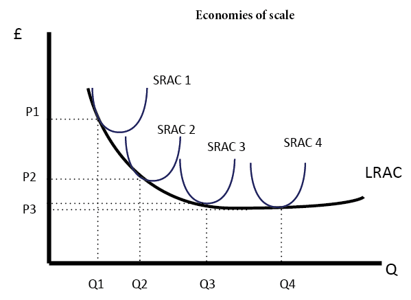
Law of Diminishing Marginal Returns Definition Diminishing marginal returns are an effect of increasing input in the short-run, while at least one production variable is kept constant, such as labor or capital. Returns to scale, on the other... › terms › dDiseconomies of Scale Definition Jan 01, 2021 · Understanding Diseconomies of Scale . The diagram below illustrates a diseconomy of scale. At point Q*, this firm is producing at the point of lowest average unit cost.If the firm produces more or ... Solved > 51.The first, second, and third workers employed ... D. marginal product of the first worker is 18. 52. If a variable input is added to some fixed input, beyond some point the resulting extra output will decline. This statement describes: A. economies and diseconomies of scale. B. X-inefficiency. C. the law of diminishing returns. D. the law of diminishing marginal utility. 53. Decision tree - Wikipedia Overview. A decision tree is a flowchart-like structure in which each internal node represents a "test" on an attribute (e.g. whether a coin flip comes up heads or tails), each branch represents the outcome of the test, and each leaf node represents a class label (decision taken after computing all attributes).The paths from root to leaf represent classification rules.
Laws of Production: Laws of Returns to Scale and Variable ... If, however, the production function exhibits increasing returns to scale, the diminishing returns arising from the decreasing marginal product of the variable factor (labour) may be offset, if the returns to scale are considerable. This, however, is rare. In general the productivity of a single-variable factor (ceteris paribus) is diminishing. DOC Chapter Overview 2. Marginal decisions are very important in determining profit levels. Marginal revenue and marginal cost are compared. 3. Marginal cost is a reflection of marginal product and diminishing returns. When diminishing returns begin, the marginal cost will begin its rise (Figure 22.6 illustrates this). 4. The marginal cost is related to AVC and ATC. The Law of Diminishing Returns: Definition, Explanation ... Stage II: Diminishing Returns. Throughout the stage of diminishing returns, the total product keeps on increasing. However unlike the stage of increasing returns, here the total product increases at a diminishing rate. This happens because the marginal product falls and becomes less than the average product, which also sees a downwards slope. PDF AGEC 105 Test 2 Fall 2012 KEY - Texas A&M University The following diagram pertains to the quantity of snack foods produced per day by Frito Lay, using labor as an input. Using the diagram, answer questions 7 - 11. 5,000 4,000 3,000 2,000 2 4 8 12 7. The marginal physical product between points B and C is: a. 500 products per hour b. 675 products per hour
Law of Diminishing Returns - an overview | ScienceDirect Topics
AmosWEB is Economics: Encyclonomic WEB*pedia The correspondence between the marginal product and marginal cost curves indicates that the law of diminishing marginal returns is the key reason for increasing marginal cost. This further implies that the law of supply and the positively-sloped supply curve can be explained in the short run by increasing marginal cost.

Indifference Curves - Overview, Diminishing Marginal Utility ...
Microeconomics Exam 2: Chapter 9 Flashcards - Quizlet In the diagram, the range of diminishing marginal returns is: D. Q1Q3. 3. In the diagram, total product will be at a maximum at: ... B. 9. 5. Use the following data to answer the question: Refer to the data. Diminishing returns begin to occur with the hiring of the _____ unit of labor. C. third. 6. Use the following data to answer the question:

Diminishing Marginal Benefit of the National Parks and ...
micro econ ch. 9 - Subjecto.com Marginal product: may initially increase, then diminish, and ultimately become negative. The law of diminishing returns describes the: relationship between resource inputs and product outputs in the short run. The total output of a firm will be at a maximum where: MP is zero. In the diagram, the range of diminishing marginal returns is: Q1Q3.
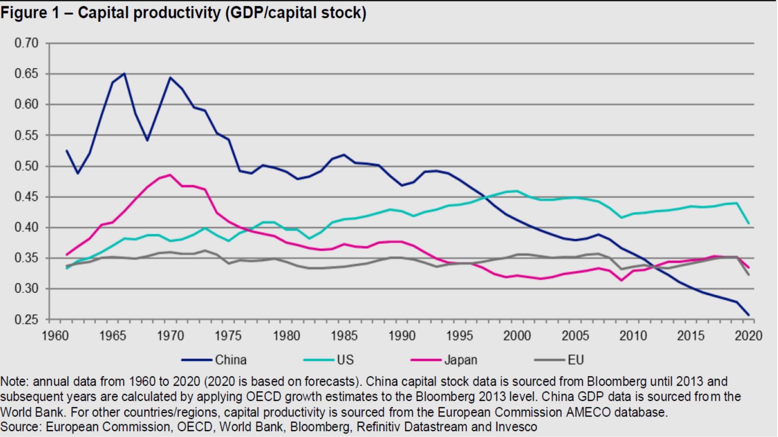
Uncommon truths: Is China over-investing?
Economic Efficiency and Pareto Optimality: Marginal ... ADVERTISEMENTS: Economic Efficiency and Pareto Optimality: Marginal Condition and Critical Evaluation! Notion of Pareto Optimality and Economic Efficiency: Economists defined social welfare as a sum total of cardinally measurable utilities of different members of the society. An optimum allocation of resources was one which maximised the social welfare in this sense. …
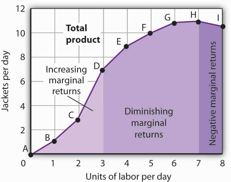
8.1 Production Choices and Costs: The Short Run – Principles ...
Average Cost and Marginal Cost (With Diagrams) According to the law of constant returns when a firm employs more and more factors, output increases at a constant rate. Therefore, the average cost curve as well as marginal cost curve remains parallel to horizontal axis. This can be made clear with the help of diagram 13. In the diagram 13 output has been measured on OX- axis while costs on ...
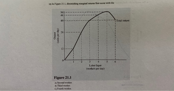
Solved 10) In Figure 21.1, diminishing marginal returns ...
37 the total output of a firm will be at a ... - Course Hero Refer to the above data. The marginal product of the fourth worker: A. is 5. B. is 7. C. is 7 1 / 2 D. cannot be calculated from the information given. negative.. 39. In the above diagram the range of diminishing marginal returns is: A. 0 Q 3 B. 0 Q 2 C. Q 1 Q 2 D. Q 1 Q 3. change in total cost that results from producing one more unit of output.

Beginners' Guide to the Law of Diminishing Returns
Solved 13. In the diagram below, the range of diminishing ... In the diagram below, the range of diminishing marginal returns is: А. 00з. В. О2. C. Qi2 D. Qi Marginal Product Average Product Q2 Inputs of Labor o Marginal and Average Product Refer to the short-run graph data below. The profit-maximizing output for this firm is A. above 440 units B. 440 units C. 320 units D. 100 units Total Cost Total $1,400
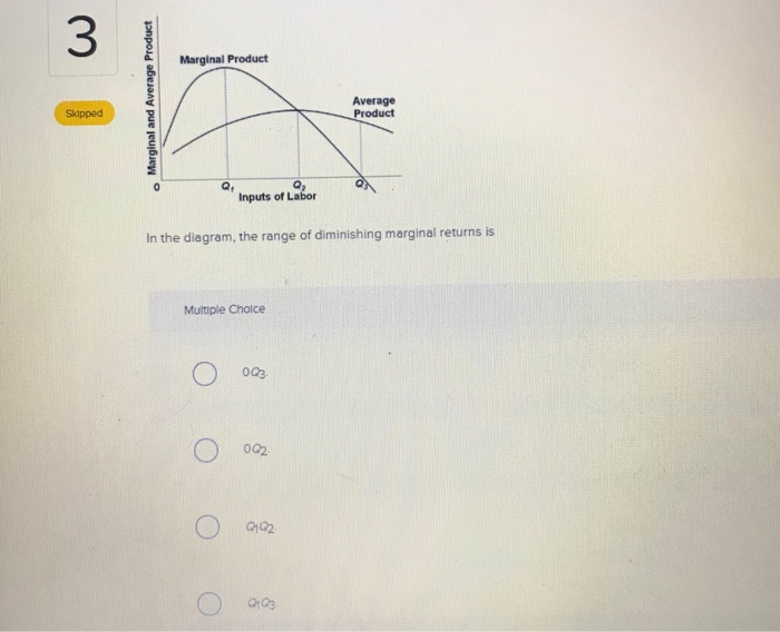
Solved Which of the following is correct 2 Multiple Choice ...
Answered: A firm produces good Y with just 2… | bartleby b) Sketch TP, AP and MP in one diagram. c) Identify the stages of production in the diagram. d) Explain why the firm still hire labour even though it is in the range of diminishing returns? e) What is the number of workers after which diminishing marginal returns starts?. f) Is this a short run or long run phenomenon?
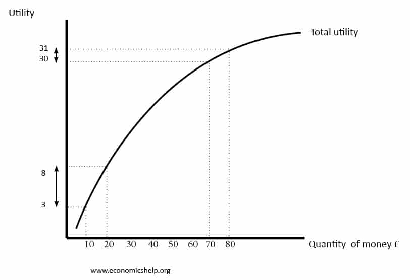
Diminishing marginal utility of income and wealth - Economics ...
PDF Midterm Questions and Answers - College of Arts and Sciences Answer: False. In fact, if a production function exhibits constant returns to scale, it must also exhibit diminishing marginal returns to labor. For example, suppose 1 typist on 1 computer produces 1 unit of output. If we have 2 typists on 2 computers, we have double the output. This is constant returns to scale.
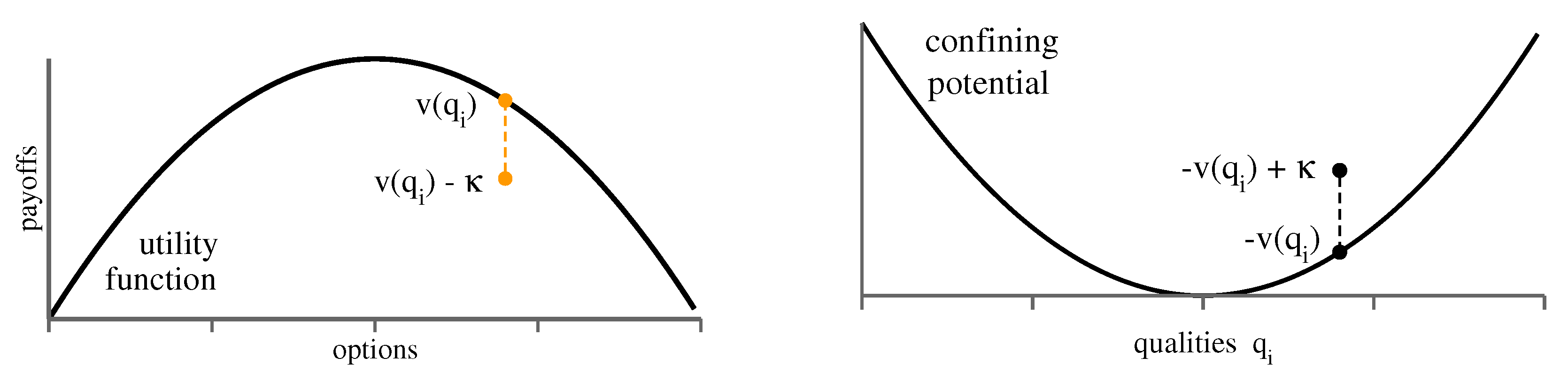
Entropy | Free Full-Text | Collective Strategy Condensation ...
Free Essay: Explain and Illustrate with ... - StudyMode Q (1) Explain and illustrate with diagrams the differences between diminishing marginal returns and decreasing economies of scale and cite causes and examples. Ans. The law of diminishing returns is also called the law of variable proportion, as the proportions of each factor of production employed keep changing as more of one factor is added.

What is Diminishing Marginal Returns, Why Does It Occur ...
Answered: Identify the stages of production in… | bartleby A firm produces good Y with just 2 factors: Capital which is fixed in supply and labour which is variable. Identify the stages of production in the diagram and explain why the firm still hire labour even though it is in the range of diminishing returns.
Costs of Production
The law of diminishing returns describes the Version 1 45 ... The law of diminishing returns describes the Version 1 45 solutiontestbankcom A. The law of diminishing returns describes the version. ... In the diagram, the range of diminishing marginal returns is A) 0 Q 3 B) 0 Q 2 C) Q 1 Q 2 D) Q 1 Q 3.... D . Q 1 Q 3 . Version 1 48. solutiontestbank.com 89) A) Q 3 units of labor.

Define Law of Diminishing Returns and its application to ...
Production Function Geometry with 'Knightian' Total Product then diminishing marginal returns to employment of the variable input(s). Although it seems reasonable that a temporary range of increasing returns to vari-able inputs will likely occur as variable inputs are added to a set of fixed ones. This proposition implies an isoquant diagram that is not a familiar one in text-books.
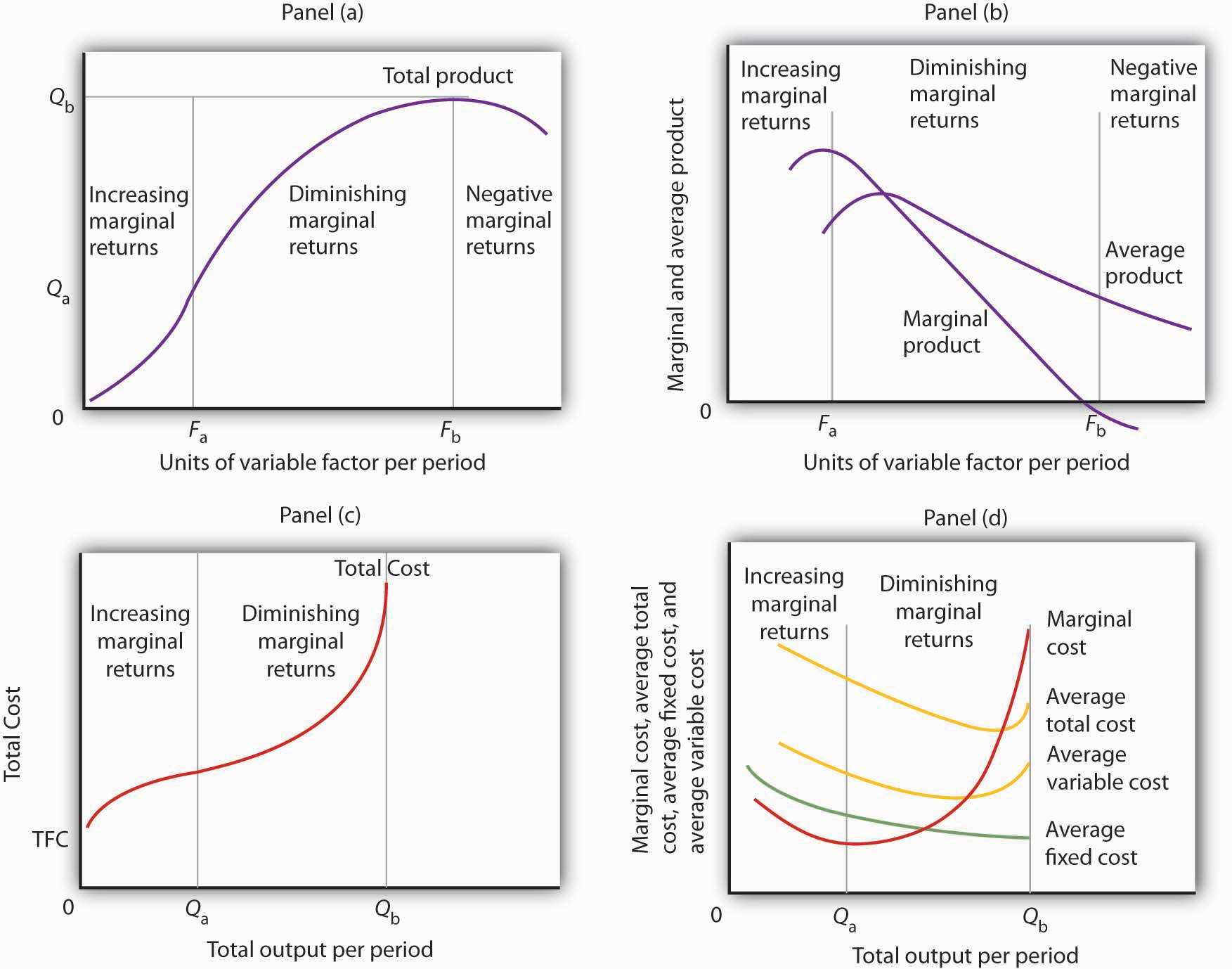
8.1 Production Choices and Costs: The Short Run – Principles ...
Law of Diminishing Returns & Point of Diminishing Returns ... It is known as the point of diminishing returns. At such a point, the marginal output is maximized but will decrease if the units of a production factor continue to increase. As the diagram above shows, the point of diminishing return is at L2.
Solved In the diagram, the range of diminishing marginal ...
Law of Diminishing Returns (Explained With Diagram) Law of Diminishing Returns (Explained With Diagram) Law of diminishing returns explains that when more and more units of a variable input are employed on a given quantity of fixed inputs, the total output may initially increase at increasing rate and then at a constant rate, but it will eventually increase at diminishing rates. In other words ...

Econ thing. Flashcards | Quizlet
The Production Process (With Diagram) - Economics Discussion Over this range marginal product is diminishing. 4. Finally, a point will be reached beyond which total output itself will actually fall, indicating a negative marginal product. In Fig. 13.4, this occurs for employment levels greater than 5.6. iii. The Average-Marginal Relationship: There is also a very close relation between MP L and AP L.
Monopsony - Overview, Advantages, Disadvantages
tutor2u | Law of Diminishing Returns, Marginal Cost and ... Diminishing returns to labour in the short run. As more of a variable factor (e.g. labour) is added to a fixed factor (e.g. capital), a firm will reach a point where it has a disproportionate quantity of labour to capital and so the marginal product of labour will fall, thus raising marginal cost and average variable cost.
Solved Question 41 Identify the range of diminishing | Chegg.com
econ exam #2 Flashcards - Quizlet In the above diagram the range of diminishing marginal returns is: Q1Q3. In the above diagram, total product will be at a maximum at: Q3 units of labor. Refer to the above diagram. At output level Q total variable cost is: ... The above diagram indicates that the marginal revenue of the sixth unit of output is. not 4.
Diminishing Marginal Return | Data Charts & Finance Templates
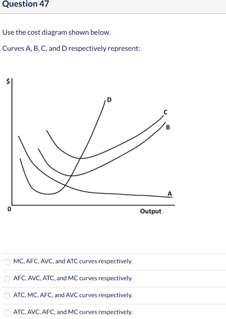
Solved Question 41 Identify the range of diminishing | Chegg.com

Law of Diminishing Returns | Central Economics Wiki | Fandom

Econ thing. Flashcards | Quizlet

Econ thing. Flashcards | Quizlet

Law of Diminishing Returns: Definition & Examples - Video ...

Unit 3 Scarcity, work, and choice – The Economy

Law of Diminishing Returns: Definition & Examples - Video ...

AmosWEB is Economics: Encyclonomic WEB*pedia
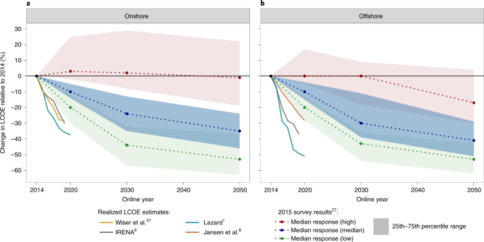
Expert elicitation survey predicts 37% to 49% declines in ...
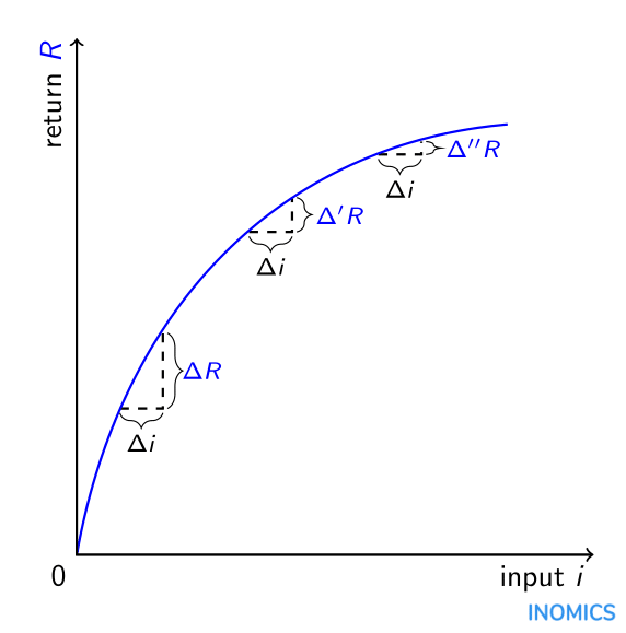
INOMICS
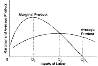
Solved In the diagram above, the range of diminishing | Chegg.com
The Law of Diminishing Marginal Returns - Economics Help

Solved Refer to the figure below. Diminishing marginal ...

Altruism or diminishing marginal utility? - ScienceDirect

Aerosols in current and future Arctic climate | Nature ...
14.02 Fall 2018 Problem Set 3 Solutions

Law of Diminishing Marginal Productivity Definition

Diminishing Marginal Utility - an overview | ScienceDirect Topics

Law of Diminishing Returns - an overview | ScienceDirect Topics
The Law of Diminishing Marginal Returns - Video & Lesson ...


Comments
Post a Comment